Reinforcement Learning is a type of Machine Learning where an agent learns to make decisions by interacting with an environment. It is based on the concept of trial and error learning, where the agent tries different actions and learns from the feedback it receives in the form of rewards or penalties. Reinforcement Learning is widely used in various domains such as gaming, robotics, finance, and healthcare.
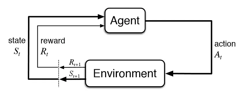 |
| Reinforcement Learning Cycle |
The Reinforcement Learning process starts with an agent and an environment. The agent interacts with the environment by taking actions and receiving feedback in the form of rewards or penalties. The goal of the agent is to maximize its cumulative reward over a period of time. The agent uses a policy, which is a set of rules that determine the actions it takes in different situations. The policy is learned through trial and error, and it is updated based on the feedback received from the environment.
The rewards and penalties in Reinforcement Learning are used to guide the agent towards making better decisions. The rewards are positive feedback that the agent receives when it takes an action that leads to a desirable outcome. The penalties, on the other hand, are negative feedback that the agent receives when it takes an action that leads to an undesirable outcome. The agent uses these feedback signals to update its policy and improve its decision-making capabilities.
One of the most important aspects of Reinforcement Learning is the exploration-exploitation trade-off. The agent needs to balance between exploring new actions and exploiting its current knowledge to maximize its reward. If the agent only exploits its current knowledge, it may miss out on better options that it has not explored yet. On the other hand, if the agent only explores new options, it may take a long time to converge to an optimal solution. The exploration-exploitation trade-off is a delicate balance that needs to be carefully managed by the agent.
There are several algorithms used in Reinforcement Learning, such as Q-learning, SARSA, and Deep Reinforcement Learning. Q-learning is a model-free algorithm that learns the optimal policy through trial and error. SARSA is another model-free algorithm that learns the optimal policy by exploring the environment and updating the policy based on the observed rewards. Deep Reinforcement Learning is a type of Reinforcement Learning that uses deep neural networks to learn complex policies in high-dimensional environments.
Now, let’s look at some of the algorithms in detail:
Q-Learning
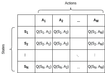
Q-learning is a reinforcement learning algorithm that is used to learn the optimal policy in a Markov decision process (MDP). It is a model-free approach that learns the optimal policy by iteratively updating the Q-values of each state-action pair in the MDP.
In Q-learning, the agent learns a Q-function that estimates the expected reward of taking a particular action in a particular state. The Q-function is defined as Q(s, a), where s is the state and a is the action. The Q-function represents the expected cumulative reward that the agent will receive by taking the action a in the state s and then following the optimal policy from that point on.
The Q-values are updated using the following update rule:
where Q(s, a) is the Q-value for taking action a in state s, α is the learning rate, r is the reward received for taking action a in state s, γ is the discount factor, max(Q(s', a')) is the maximum Q-value for any action a' in the next state s', and s' is the state that results from taking action a in state s.
The update rule is based on the Bellman equation, which states that the optimal Q-value for a state-action pair is equal to the expected reward of taking that action plus the expected reward of following the optimal policy from that point on. The update rule uses the difference between the expected reward and the current Q-value to update the Q-value of the state-action pair.
The Q-learning algorithm starts with an initial Q-function, which may be set to zero or some arbitrary value. The agent then interacts with the environment, selecting actions based on the current Q-function and receiving rewards in return. The Q-values are updated after each action, and the process is repeated until the Q-function converges to the optimal policy.
 |
| Q-Table |
One of the key advantages of Q-learning is that it can handle environments with a large or continuous state space. The Q-function can be represented using a lookup table, a neural network, or other function approximators, depending on the complexity of the environment. Q-learning can also handle delayed rewards and can learn from experience, making it suitable for a wide range of applications.
However, Q-learning also has some limitations. It requires a lot of data to learn the optimal policy, which may be time-consuming and expensive. It also requires careful management of the exploration-exploitation trade-off to avoid getting stuck in local optima. Finally, Q-learning may not perform well in environments where the state transitions are non-Markovian or where the reward function is poorly defined.
In conclusion, Q-learning is a powerful reinforcement learning algorithm that can be used to learn the optimal policy in a wide range of environments. It is based on the concept of learning the Q-values for each state-action pair and using the Bellman equation to update the Q-values iteratively. Q-learning has several advantages over other reinforcement learning algorithms, such as its ability to handle large or continuous state spaces and delayed rewards. However, it also has some limitations that need to be carefully managed.
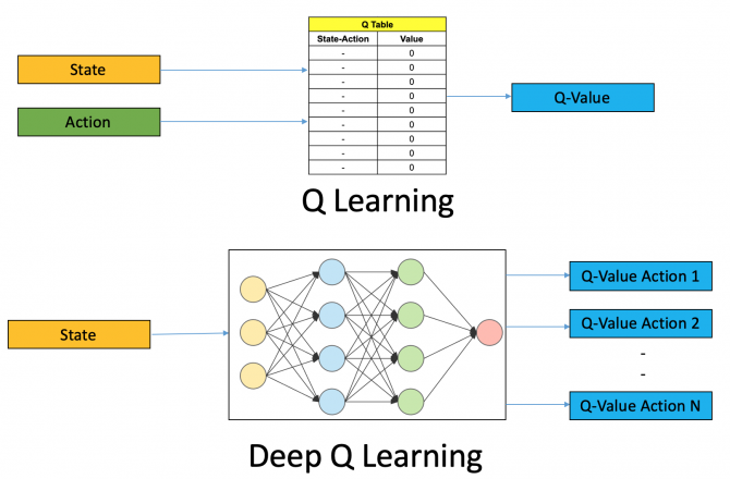
Deep Q-Learning
Deep Q-Learning (DQL) is a type of reinforcement learning algorithm that combines Q-Learning, a model-free algorithm, with deep neural networks. It is used to learn optimal policies in complex and high-dimensional environments.
In DQL, the Q-function, which estimates the expected cumulative reward of taking an action in a given state and following a certain policy, is represented by a deep neural network. The input to the network is the state, and the output is a vector of Q-values for each possible action in that state. The optimal policy is derived from the action with the highest Q-value.
 |
| Q-Learning v/s Deep Q-Learning |
The algorithm uses an experience replay buffer to store transitions (s, a, r, s') observed during the interaction of the agent with the environment. The replay buffer is used to sample batches of transitions randomly to break the correlation between consecutive transitions and improve learning stability.
DQL uses a target network to update the Q-function. The target network is a copy of the Q-network that is used to evaluate the Q-value of the next state in the Bellman equation, which defines the optimal Q-function. The target network is updated periodically by copying the weights from the Q-network.
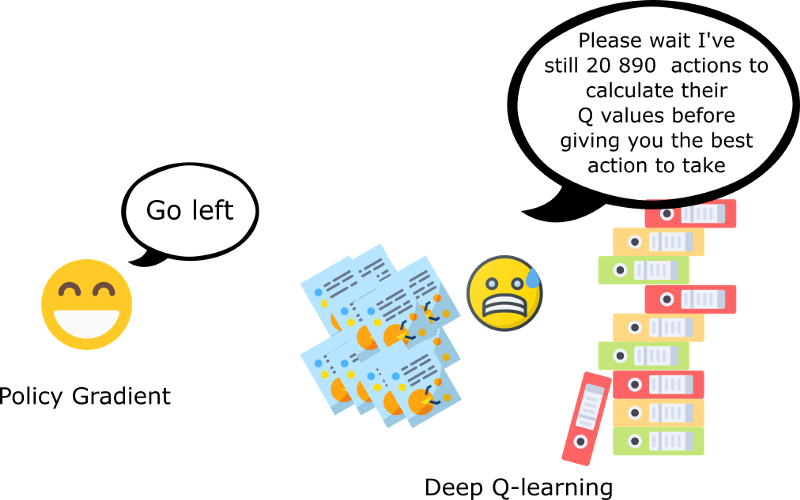
Policy Gradients
Policy Gradients is a reinforcement learning algorithm that aims to learn a stochastic policy that maximizes the expected cumulative reward in a Markov decision process (MDP). Unlike value-based methods, such as Q-learning and SARSA, which learn the optimal Q-value function or state-action values, Policy Gradients directly learn the policy function that maps states to actions.
 |
| Policy Gradient |
The Policy Gradients algorithm uses a gradient ascent approach to iteratively improve the policy by maximizing the expected cumulative reward. The algorithm updates the policy parameters in the direction of the gradient of the expected cumulative reward with respect to the policy parameters. The update rule is given by:
where θ is the policy parameter, α is the learning rate, and J(θ) is the objective function, which is defined as the expected cumulative reward over a trajectory:
where R is the cumulative reward over a trajectory and πθ is the policy function parameterized by θ.
The gradient of the objective function can be computed using the score function estimator:
where T is the time horizon of the trajectory, st and at are the state and action at time t, and R is the cumulative reward over the trajectory.
The Policy Gradients algorithm also uses a baseline function, which is a function that estimates the expected cumulative reward under the current policy. The baseline function is subtracted from the cumulative reward to reduce the variance of the gradient estimator.
The baseline function can be any function that depends only on the state, such as a state-value function, a constant value, or a function of the state features. The baseline function can be learned jointly with the policy parameters, or it can be estimated separately using a supervised learning or regression algorithm.
One of the advantages of Policy Gradients is that it can handle environments with continuous state and action spaces, and it can learn stochastic policies that can explore the state-action space more effectively. Another advantage is that it can optimize non-differentiable objectives, such as the expected cumulative reward.
However, Policy Gradients suffers from high variance in the gradient estimator, which can lead to slow convergence and unstable learning. To address this issue, several techniques have been proposed, such as the use of trust regions, natural policy gradients, actor-critic methods, and importance sampling.
In conclusion, Policy Gradients is a powerful reinforcement learning algorithm that learns a stochastic policy that maximizes the expected cumulative reward in a Markov decision process (MDP). The algorithm updates the policy parameters in the direction of the gradient of the expected cumulative reward with respect to the policy parameters, using a score function estimator. Policy Gradients can handle environments with continuous state and action spaces, and it can optimize non-differentiable objectives. However, it suffers from high variance in the gradient estimator, which can be addressed by using variance reduction techniques.
Proximal Policy Optimization
Proximal Policy Optimization (PPO) is a reinforcement learning algorithm that learns a stochastic policy that maximizes the expected cumulative reward in a Markov decision process (MDP). PPO belongs to the family of policy gradient methods and is designed to address the problem of high variance in gradient estimation that occurs in standard policy gradient methods.
The core idea of PPO is to update the policy parameters in a way that is "proximal" to the current policy, meaning that the update does not deviate too far from the current policy. This helps to ensure stability and prevent catastrophic updates that could harm the performance of the policy.
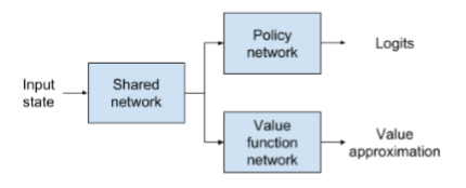 |
| Components of PPO |
The PPO algorithm consists of two key components: a clipped surrogate objective and a value function. The clipped surrogate objective is used to update the policy parameters, while the value function is used to estimate the expected cumulative reward under the current policy.
The clipped surrogate objective is given by:
where θ is the policy parameter, A is the advantage function, which measures the advantage of taking a particular action in a given state, and ratio(θ) is the ratio of the probability of taking the action under the new policy to the probability of taking the action under the old policy. The ratio is used to compute the advantage-weighted gradient, which is clipped to ensure that the update does not deviate too far from the current policy.
The value function is used to estimate the expected cumulative reward under the current policy. The value function is learned using a supervised learning or regression algorithm, such as a neural network, and is updated using the mean-squared error between the predicted value and the actual value.
The PPO algorithm updates the policy parameters and the value function iteratively using stochastic gradient descent (SGD). At each iteration, a batch of trajectories is collected using the current policy, and the clipped surrogate objective and value function are optimized using the batch data. The policy parameters and the value function are updated separately, but they can share the same neural network architecture.
One of the advantages of PPO is that it is more stable and efficient than standard policy gradient methods, such as REINFORCE and TRPO, because it uses a clipped surrogate objective that prevents large updates and catastrophic forgetting. PPO is also robust to hyperparameter tuning and can handle environments with high-dimensional state and action spaces.
Soft Actor Critic (SAC)
The Soft Actor-Critic (SAC) model is a reinforcement learning algorithm that learns a stochastic policy that maximizes the expected cumulative reward in a Markov decision process (MDP). Unlike Q-learning, which learns a Q-function, SAC learns a policy directly by maximizing the expected cumulative reward.
The SAC model has two main components: a soft actor and a critic. The soft actor is a stochastic policy that maps states to probability distributions over actions. The critic estimates the value function of the policy, which represents the expected cumulative reward that the agent will receive by following the policy.
 |
| Soft Actor Critic |
The SAC algorithm optimizes the policy by iteratively updating the parameters of the soft actor and critic. The update rule for the soft actor is based on the maximum entropy principle, which encourages the policy to explore the state-action space and avoid getting stuck in local optima. The update rule for the critic is based on the Bellman equation, which estimates the expected cumulative reward of following the policy from each state.
The update rule for the soft actor is given by:
where θ is the parameter of the soft actor, α is the learning rate, Qϕ(s,a) is the Q-value of taking action a in state s, β is the temperature parameter that controls the entropy regularization term, and H(πθ) is the entropy of the policy πθ.
The update rule for the critic is given by:
where ϕ is the parameter of the critic, r is the reward received for taking action a in state s, γ is the discount factor, Vϕ'(s') is the value function of the target network, and Vϕ(s) is the value function of the critic.
The SAC algorithm also uses a replay buffer to store transitions and samples from the buffer to update the soft actor and critic. The replay buffer helps to decorrelate the data and improve the stability of the learning process.
One of the key advantages of SAC is that it can handle environments with continuous state and action spaces. The soft actor can learn a stochastic policy that maps states to probability distributions over actions, which allows it to explore the state-action space more effectively. The entropy regularization term in the update rule also encourages exploration and helps to avoid getting stuck in local optima.
In conclusion, the Soft Actor-Critic (SAC) model is a powerful reinforcement learning algorithm that learns a stochastic policy that maximizes the expected cumulative reward in a Markov decision process (MDP). It has two main components: a soft actor that maps states to probability distributions over actions and a critic that estimates the value function of the policy. The update rules for the soft actor and critic are based on the maximum entropy principle and the Bellman equation, respectively. The SAC algorithm can handle environments with continuous state and action spaces and encourages exploration by using the entropy regularization term.
Advantages and Limitations
Reinforcement Learning has several advantages over other Machine Learning approaches. It can handle complex environments where the state space is large or continuous. It can also handle environments with delayed rewards, where the agent may have to make decisions that only affect the reward in the long term. Reinforcement Learning can also learn from experience and adapt to changing environments.
However, Reinforcement Learning also has some limitations. It requires a lot of data to learn an optimal policy, which may be time-consuming and expensive. It also requires careful management of the exploration-exploitation trade-off, which may be challenging in some environments. Finally, the performance of Reinforcement Learning algorithms may depend on the quality of the reward function, which may be difficult to design in some domains.
Conclusion
In conclusion, Reinforcement Learning is a powerful approach to Machine Learning that has shown impressive results in various domains. It is based on the concept of trial and error learning, where an agent learns to make decisions by interacting with an environment and receiving feedback in the form of rewards or penalties. Reinforcement Learning has several advantages over other Machine Learning approaches, such as its ability to handle complex environments and delayed rewards. However, it also has some limitations that need to be carefully managed.
Comments
Post a Comment